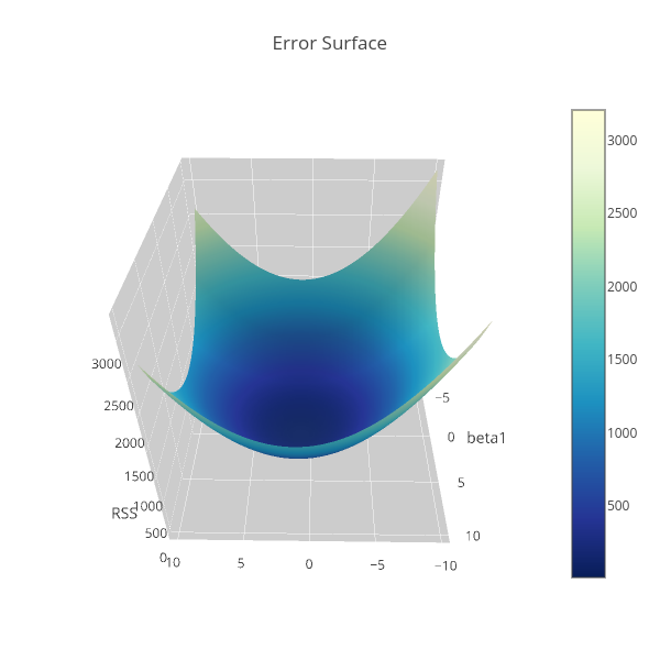
In my previous article, we talked about implementations of linear regression models in R, Python and SAS. On the theoretical sides, however, I briefly mentioned the estimation procedure for the parameter $boldsymbol{beta}$. So to help us understand how software does the estimation procedure, we’ll look at the mathematics behind it. We will also perform the estimation manually in R and in Python, that means we’re not gonna use any special packages, this will help us appreciate the theory.
Linear Least Squares
Consider the linear regression model, [ y_i=f_i(mathbf{x}|boldsymbol{beta})+varepsilon_i,quadmathbf{x}_i=left[ begin{array}{cccc} 1&x_{11}&cdots&x_{1p} end{array}right],quadboldsymbol{beta}=left[begin{array}{c}beta_0beta_1vdotsbeta_pend{array}right], ] where $y_i$ is the response or the dependent variable at the $i$th case, $i=1,cdots, N$. The $f_i(mathbf{x}|boldsymbol{beta})$ is the deterministic part of the model that depends on both the parameters $boldsymbol{beta}inmathbb{R}^{p+1}$ and the predictor variable $mathbf{x}_i$, which in matrix form, say $mathbf{X}$, is represented as follows [ mathbf{X}=left[ begin{array}{cccccc} 1&x_{11}&cdots&x_{1p} 1&x_{21}&cdots&x_{2p} vdots&vdots&ddots&vdots 1&x_{N1}&cdots&x_{Np} end{array} right]. ] $varepsilon_i$ is the error term at the $i$th case which we assumed to be Gaussian distributed with mean 0 and variance $sigma^2$. So that [ mathbb{E}y_i=f_i(mathbf{x}|boldsymbol{beta}), ] i.e. $f_i(mathbf{x}|boldsymbol{beta})$ is the expectation function. The uncertainty around the response variable is also modelled by Gaussian distribution. Specifically, if $Y=f(mathbf{x}|boldsymbol{beta})+varepsilon$ and $yin Y$ such that $y>0$, then begin{align*} mathbb{P}[Yleq y]&=mathbb{P}[f(x|beta)+varepsilonleq y] &=mathbb{P}[varepsilonleq y-f(mathbf{x}|boldsymbol{beta})]=mathbb{P}left[frac{varepsilon}{sigma}leq frac{y-f(mathbf{x}|boldsymbol{beta})}{sigma}right] &=Phileft[frac{y-f(mathbf{x}|boldsymbol{beta})}{sigma}right], end{align*} where $Phi$ denotes the Gaussian distribution with density denoted by $phi$ below. Hence $Ysimmathcal{N}(f(mathbf{x}|boldsymbol{beta}),sigma^2)$. That is, begin{align*} frac{operatorname{d}}{operatorname{d}y}Phileft[frac{y-f(mathbf{x}|boldsymbol{beta})}{sigma}right]&=phileft[frac{y-f(mathbf{x}|boldsymbol{beta})}{sigma}right]frac{1}{sigma}=mathbb{P}[y|f(mathbf{x}|boldsymbol{beta}),sigma^2] &=frac{1}{sqrt{2pi}sigma}expleft{-frac{1}{2}left[frac{y-f(mathbf{x}|boldsymbol{beta})}{sigma}right]^2right}. end{align*} If the data are independent and identically distributed, then the log-likelihood function of $y$ is, begin{align*} mathcal{L}[boldsymbol{beta}|mathbf{y},mathbf{X},sigma]&=mathbb{P}[mathbf{y}|mathbf{X},boldsymbol{beta},sigma]=prod_{i=1}^Nfrac{1}{sqrt{2pi}sigma}expleft{-frac{1}{2}left[frac{y_i-f_i(mathbf{x}|boldsymbol{beta})}{sigma}right]^2right} &=frac{1}{(2pi)^{frac{n}{2}}sigma^n}expleft{-frac{1}{2}sum_{i=1}^Nleft[frac{y_i-f_i(mathbf{x}|boldsymbol{beta})}{sigma}right]^2right} logmathcal{L}[boldsymbol{beta}|mathbf{y},mathbf{X},sigma]&=-frac{n}{2}log2pi-nlogsigma-frac{1}{2sigma^2}sum_{i=1}^Nleft[y_i-f_i(mathbf{x}|boldsymbol{beta})right]^2. end{align*} And because the likelihood function tells us about the plausibility of the parameter $boldsymbol{beta}$ in explaining the sample data. We therefore want to find the best estimate of $boldsymbol{beta}$ that likely generated the sample. Thus our goal is to maximize the likelihood function which is equivalent to maximizing the log-likelihood …read more
Source:: r-bloggers.com
