(This article was originally published at Analysis with Programming, and syndicated at StatsBlogs.)
In my previous article, we talked about implementations of linear regression models in R, Python and SAS. On the theoretical sides, however, I briefly mentioned the estimation procedure for the parameter $boldsymbol{beta}$. So to help us understand how software does the estimation procedure, we’ll look at the mathematics behind it. We will also perform the estimation manually in R and in Python, that means we’re not gonna use any special packages, this will help us appreciate the theory.
Linear Least Squares
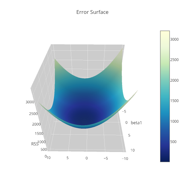
Consider the linear regression model, [ y_i=f_i(mathbf{x}|boldsymbol{beta})+varepsilon_i,quadmathbf{x}_i=left[ begin{array}{cccc} 1&x_{11}&cdots&x_{1p} end{array}right],quadboldsymbol{beta}=left[begin{array}{c}beta_0beta_1vdotsbeta_pend{array}right], ] where $y_i$ is the response or the dependent variable at the $i$th case, $i=1,cdots, N$. The $f_i(mathbf{x}|boldsymbol{beta})$ is the deterministic part of the model that depends on both the parameters $boldsymbol{beta}inmathbb{R}^{p+1}$ and the predictor variable $mathbf{x}_i$, which in matrix form, say $mathbf{X}$, is represented as follows [ mathbf{X}=left[ begin{array}{cccccc} 1&x_{11}&cdots&x_{1p} 1&x_{21}&cdots&x_{2p} vdots&vdots&ddots&vdots 1&x_{N1}&cdots&x_{Np} end{array} right]. ] $varepsilon_i$ is the error term at the $i$th case which we assumed to be Gaussian distributed with mean 0 and variance $sigma^2$. So that [ mathbb{E}y_i=f_i(mathbf{x}|boldsymbol{beta}), ] i.e. $f_i(mathbf{x}|boldsymbol{beta})$ is the expectation function. The uncertainty around the response variable is also modelled by Gaussian distribution. Specifically, if $Y=f(mathbf{x}|boldsymbol{beta})+varepsilon$ and $yin Y$ such that $y>0$, then begin{align*} mathbb{P}[Yleq y]&=mathbb{P}[f(x|beta)+varepsilonleq y] &=mathbb{P}[varepsilonleq y-f(mathbf{x}|boldsymbol{beta})]=mathbb{P}left[frac{varepsilon}{sigma}leq frac{y-f(mathbf{x}|boldsymbol{beta})}{sigma}right] &=Phileft[frac{y-f(mathbf{x}|boldsymbol{beta})}{sigma}right], end{align*} where $Phi$ denotes the Gaussian distribution with density denoted by $phi$ below. Hence $Ysimmathcal{N}(f(mathbf{x}|boldsymbol{beta}),sigma^2)$. That is, begin{align*} frac{operatorname{d}}{operatorname{d}y}Phileft[frac{y-f(mathbf{x}|boldsymbol{beta})}{sigma}right]&=phileft[frac{y-f(mathbf{x}|boldsymbol{beta})}{sigma}right]frac{1}{sigma}=mathbb{P}[y|f(mathbf{x}|boldsymbol{beta}),sigma^2] &=frac{1}{sqrt{2pi}sigma}expleft{-frac{1}{2}left[frac{y-f(mathbf{x}|boldsymbol{beta})}{sigma}right]^2right}. end{align*} If the data are independent and identically distributed, then the log-likelihood function of $y$ is, begin{align*} mathcal{L}[boldsymbol{beta}|mathbf{y},mathbf{X},sigma]&=mathbb{P}[mathbf{y}|mathbf{X},boldsymbol{beta},sigma]=prod_{i=1}^Nfrac{1}{sqrt{2pi}sigma}expleft{-frac{1}{2}left[frac{y_i-f_i(mathbf{x}|boldsymbol{beta})}{sigma}right]^2right} &=frac{1}{(2pi)^{frac{n}{2}}sigma^n}expleft{-frac{1}{2}sum_{i=1}^Nleft[frac{y_i-f_i(mathbf{x}|boldsymbol{beta})}{sigma}right]^2right} logmathcal{L}[boldsymbol{beta}|mathbf{y},mathbf{X},sigma]&=-frac{n}{2}log2pi-nlogsigma-frac{1}{2sigma^2}sum_{i=1}^Nleft[y_i-f_i(mathbf{x}|boldsymbol{beta})right]^2. end{align*} And because the likelihood function tells us about the plausibility of the parameter $boldsymbol{beta}$ in explaining the sample data. We therefore want to find the best estimate of $boldsymbol{beta}$ that likely generated the sample. Thus our goal is …read more
Source:: statsblogs.com
